Thickness Mapping of a Draining Soap Film

Introduction

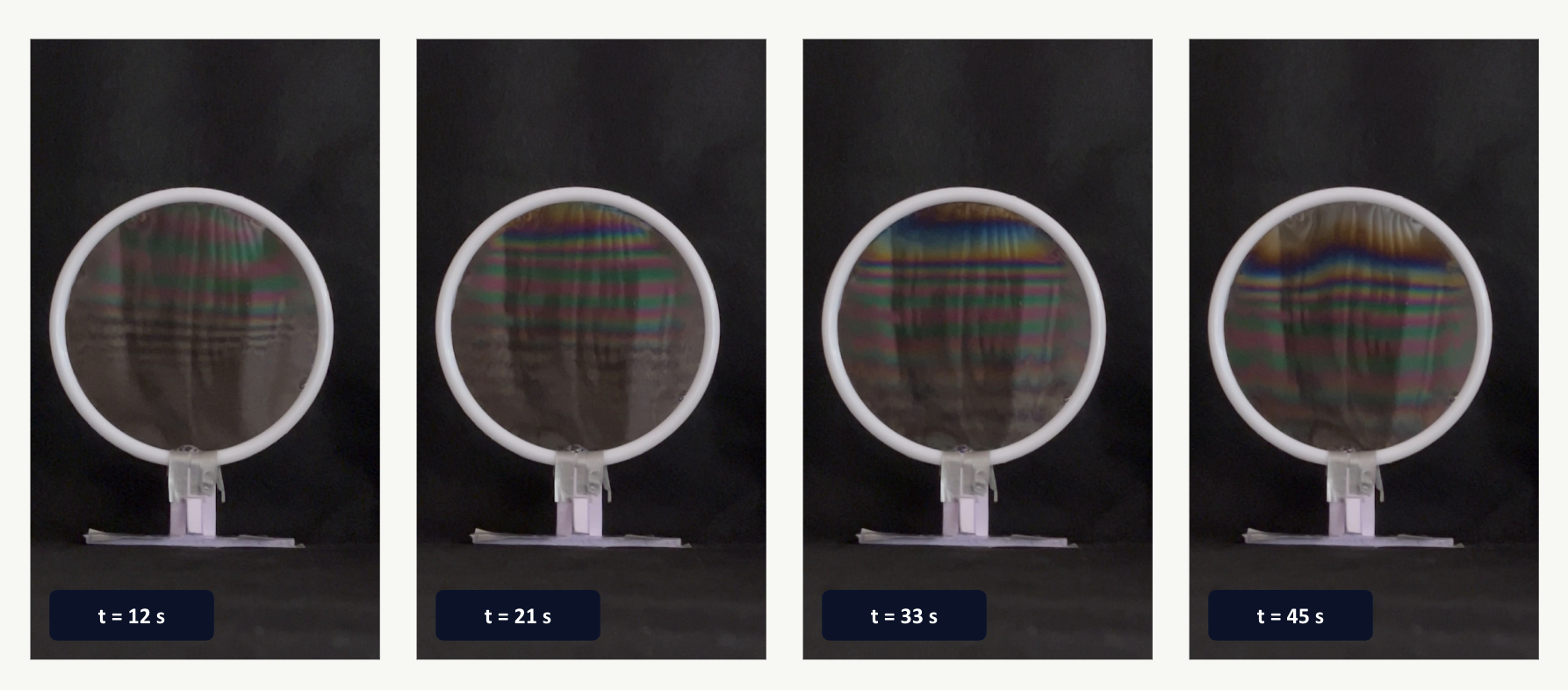
Soap films are one of the few places where wave optics become visible to the naked eye. Put a thin soap film under a light source, and you will observe a beautiful color pattern, evolving over time. This process is the drainage of the film(as a result of gravity), and the colors themselves secretly encode the thickness of the film at that given region(down to nanometers). Using some simple optical physics, we can recover the thickness of the film over time, as the film drains.

The process used to drive this project is described in a 2025 paper by Carlà, Molesini, and Straulino in the American Journal of Physics, which uses draining soap films as a teaching tool for interference and color science. I wanted to replicate their approach experimentally and then push it further: build an automated pipeline that could take a raw video of a draining film and turn it into a quantitative thickness-vs-time dataset, without any manual frame-by-frame work.

The Challenge

The underlying physics is straightforward in principle: light reflects off both the front and back surface of the film, the two reflections interfere, and the resulting color depends on the film's thickness and refractive index. The task at hand however is a little more challenging: starting from a photograph's colors and recovering the thickness that produced them.

This conversion has a fundamental ambiguity in it. The reflectance of a thin film is a sine-squared function of thickness, which means it's periodic: many different thicknesses can produce nearly the same color. A raw video frame gives you color; color alone doesn't tell you which "order" of the interference pattern you're looking at. On top of that, the actual video I recorded has practical problems a clean theoretical model doesn't: an uncalibrated camera, uneven lighting, glare, and a soap film that isn't sitting still.

So the project split into two halves that had to work together: a physics model accurate enough to generate the right colors for a given thickness, and a computer vision pipeline robust enough to invert that model on messy, real-world footage.

Physical Setup

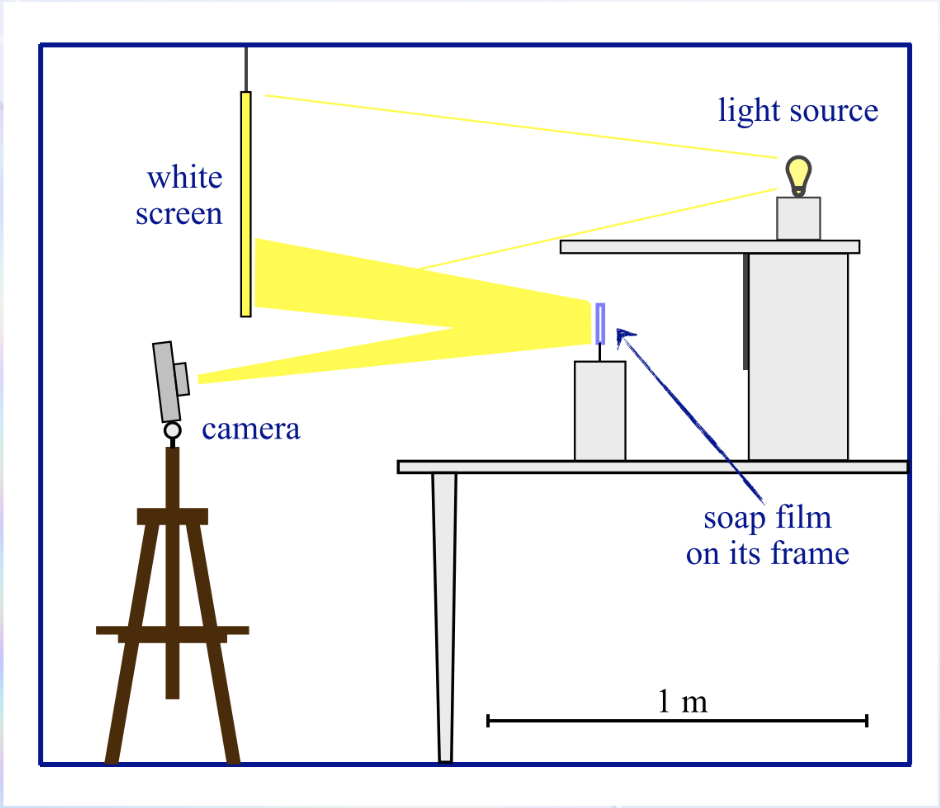
The apparatus was intentionally simple, and I built it from scratch.

• Film holder: A circular plastic ring about 11 cm in diameter, dipped in solution to form a stable, vertical soap film.
• Soap Solution: dish soap, glycerin, and water in a 2:2:5 ratio by volume. Glycerin slows evaporation and drainage, which gives the film a long enough lifetime to actually film. This mixture has a refractive index of roughly n = 1.36.
• Illumination: a single incandescent lamp, chosen because its broadband, tungsten-like spectrum is well-approximated by a Planckian (blackbody) source, which made it easy to model accurately.
• Diffuser: a sheet of PVC foam between the lamp and the film, to soften and spread the light evenly.
• Background: black felt behind the film, to suppress stray reflections and keep the interference colors high-contrast.
• Camera: a fixed, stationary camera recording the film face-on at 3840x2160 resolution, about 30 fps(IPhone 13).

An overview of the Methodology

The breakdown of the video to data process can be split into three steps:

1. Frame Extraction: Sample the raw video every 3 seconds, snapping to the nearest true frame and logging the exact timestamp.
2. Converting the Color to Thickness: Build a physics-based thickness-to-color lookup table, then invert it per-frame using chromaticity matching plus a monotonicity constraint from the drainage physics.
3. Assembly: combine every frame's thickness profile onto one graph, showing how the drainage evolves over the full roughly 50-second recording.

The Physics: Thin-Film interference

For light hitting the film close to head-on, the two surfaces reflect it, and the two reflected waves travel slightly different distances before recombining — the optical path difference, OPD = 2nd, where n is the refractive index and d is the film thickness. Whether a given wavelength interferes constructively or destructively at that thickness follows a simple two-beam model (a good approximation for a soap film in air, where multiple internal reflections are weak):

So what we see is that as \(d\) grows, the reflectance oscillates through the visible spectrum(it is the distance accumulated as we move from the top to the bottom of the ring). This is precisely why we see a repeating pattern of colors in a sequence: dark, straw, orange, magenta, blue, green, and then repeating and gradually washing out (desaturating) at greater thicknesses. Each full color cycle corresponds to one interference order: a thicker film sits at a higher order.

I used this relationship, together with the lamp's spectrum and the human eye's known color response, to build a reference table connecting each candidate thickness to the RGB color a camera would actually see.

The Code

The code for the project is broken into the three primary programs. A more in-depth walk through is viewable in my GitHub Repository for the project, but here is the basic outline:

1. Building the Color Reference Table: build_lut.py

This step doesn't touch the video at all. It's a pure physics simulation answering: for a given film thickness, what color would a camera see? For every thickness from 0-2000 nm, it computes the reflectance spectrum R(λ) = sin²(2πnd/λ), multiplies it by a modeled lamp spectrum (a 2856 K blackbody, standing in for the incandescent bulb), then converts that spectrum into an actual RGB color via the CIE 1931 standard observer: the standard model of how the human eye's three cone types respond to each wavelength. Then, it is followed by a standard XYZ→sRGB conversion. The result is a 2001-entry lookup table (LUT) pairing thickness with color, validated by checking it reproduces the well-known Newton's-colors sequence.

2. Reading the thickness out of the video: extract_thickness.py

This is the most involved script. For each frame: a Hough circle transform locates the film's ring (robust to the background's uneven brightness, which breaks simpler thresholding). The ring is shrunk inward by 12% and cropped to a central vertical strip, restricted to the top 65% of the film. Glare pixels are flagged and excluded via HSV thresholding. The remaining pixel colors are converted to chromaticity (normalized by their own brightness) so the video's uncalibrated, dim exposure doesn't bias every match toward the LUT's near-black entries. Then finally, each row's chromaticity is matched against the LUT using dynamic programming, enforcing that thickness never decreases going down the film, which is the physical signature of gravity-driven drainage This resolves the otherwise-ambiguous color matches. Each frame also gets a QC image showing exactly what was detected, for debugging.

3. Assembling the Drainage: assemble_graph.py

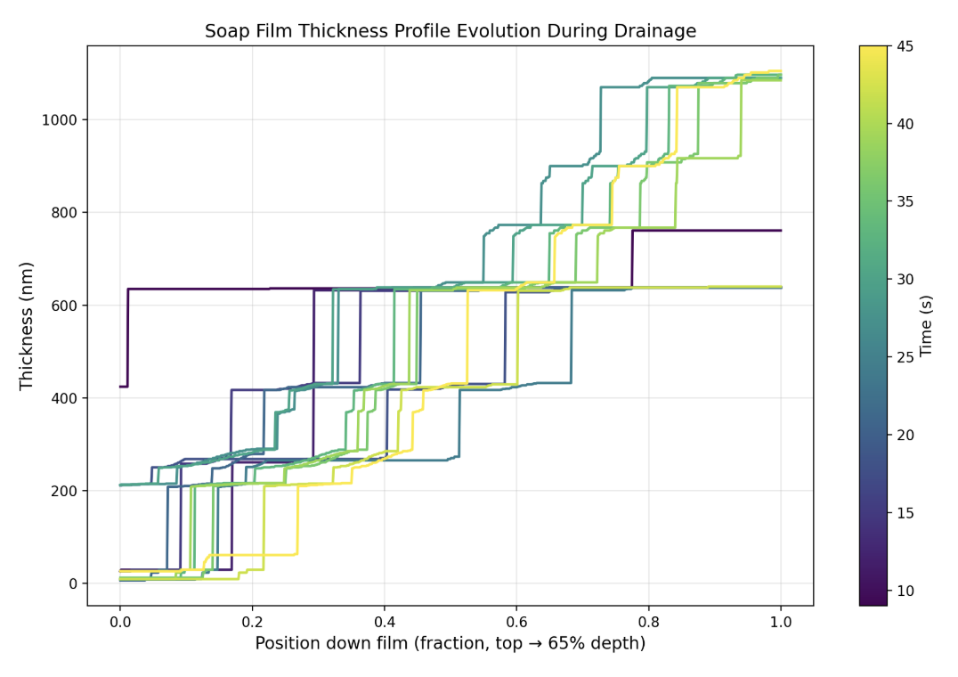
This program loads every frame's thickness profile and overlays them on one plot, colored by capture time, with a light display-only smoothing pass to remove the small "staircase" artifacts from the LUT's discrete indexing.

What I Found

Across 13 valid frames spanning the roughly 50-second recording, the process recovered a clear and physically sensible drainage trend. The maximum resolved thickness in the analyzed region grew from roughly 640-760 nm in the earliest usable frames (t = 9-24 s) up to about 1090-1100 nm by t = 27-45 s, and this is consistent with continued gravity-driven drainage thickening the lower part of the film over time.

The profiles also showed a consistent structural feature: broad, well-separated color "steps" near the top of the film, where the interference order is low, narrowing into finer, more closely-spaced steps further down as the order increases. That's exactly the qualitative result you'd expect from the underlying sine-squared reflectance model.

Two edge cases were also handled automatically, rather than silently reported as bad data. The first ~6 seconds of footage were excluded because the measured strip brightness (~24 out of 255) was well below the ~55-80 range seen once the lamp and film had settled, there simply wasn't a usable color signal yet. And the film itself ruptured by around t ≈ 48 s; the final frame showed an empty ring, which the pipeline correctly flagged and excluded rather than reporting a spurious near-zero thickness.

Where the Results Fall Short

A few limitations are worth noting in this process. Some of them are fixable with more work, while others are closer to the fundemental limits of the method:

• No absolute color calibration: I never measured the camera's exact spectral response against a known color reference. The thickness values are self-consistent within the model, but not independently verified against ground truth.
• Fundemental order ambiguity: Beyond a few interference orders, many distinct thicknesses genuinely produce very similar colors. This is a known limit of single-exposure RGB interferometry generally, not just a gap in this implementation, and it's the reason the lookup table is capped at 2000 nm
• The monotonicity assumption: Forcing thickness to increase down the film is a reasonable match for gravity-driven drainage, but it would mask any local non-monotonic features
• Coarse Temporal Sampling: Sampling every 3 seconds, which was chosen mainly for tractability, can't measure faster drainage dynamics, and it missed whatever happened in the several seconds between the last good frame and the rupture.

Conclusion and Further Improvements

So to bring everything together, this was a fun project to navigate, bringing just shining a light on a soap film into a quantitative, physics-based measurement that gave the thickness of the film in nanometers. The model held up against the known Newton's-colors sequence, and the program ran start to finish with a pure automated pipeline, producing a physically sensible drainage trend.

There is of course plenty to push this experiment further. For example, the camera could be calibrated against a known color reference to make the thickness values independently verifiable. Filming at a higher frame rate would also better allow to capture the actual rupture process, making better note of the fastest part of the drainage process. For now, only a strip of the film was analyzed to neglect effects of glare, but using a bigger portion would give stronger results. Lastly, the model could be stretched to handle more of the washed-out colors that show up as the film thickens further. Many of these things would simply require stronger instrumentation.

References

- M. Carlà, G. Molesini, and S. Straulino, “ Color and thickness of soap films ”, Am. J. Phys. 93 (11), 914-924 (2025).
- W. Wyman, P.-P. Sloan, and P. Shirley, “ Simple Analytic Approximations to the CIE XYZ Color Matching Functions ”, J. Comp. Graphics Techniques 2 (2), 1-11 (2013).
Additional Readings
- N. S. Lalli and A. Giusti, “ Coherence effects on the interference colors of soap films ”, J. Appl. Phys. 134 (9), 093103 (2023).
- Y. D. Afanasyev, G. T. Andrews, and C. G. Deacon, “ Measuring soap bubble thickness with color matching ”, Am. J. Phys. 79 (10), 1079-1082 (2011).