Machine Learning the Higgs Boson

Why I Built This

Particle physics experiments produce an enormous amount of data from collisions between particles. Hidden within these collisions are rare events that can reveal new particles and interactions, but separating those interesting events from the much larger background of ordinary collisions is a difficult problem.

The Higgs boson is a particularly interesting example. When protons collide at extremely high energies, a Higgs boson can occasionally be produced, but its presence cannot be observed directly in the detector. Instead, physicists look for the characteristic patterns left behind by its decay products and use those measurements to determine whether a collision is consistent with a Higgs event or with background processes.

I wanted to explore whether machine learning could help with this task. Rather than manually defining a small number of criteria for identifying an event, a machine learning model can learn patterns across many measurements at once. This project gave me a way to explore that idea while combining my interests in particle physics, computation, and data analysis.

The Challenge

A particle detector does not simply record an event as “Higgs” or “not Higgs.” Instead, each collision is represented by a collection of physical measurements describing what happened during the interaction. These measurements include quantities related to the particles produced in the collision, such as their momenta, angles, and energies.

The challenge was to determine whether these measurements contained enough information to distinguish signal from background. Rather than relying on one measurement at a time, the model would consider the features of an entire event simultaneously and learn which combinations were associated with Higgs-like collisions.

The challenge was to determine whether these measurements contained enough information to distinguish signal from background. Rather than relying on one measurement at a time, the model would consider the features of an entire event simultaneously and learn which combinations were associated with Higgs-like collisions.

What I Did

I approached the project as a progression from exploration to modeling and finally interpretation. I first examined the available collision variables to understand how the data differed between signal and background and to identify which measurements appeared most informative.

I then trained and compared several classification models, using their performance to determine which approach was most promising. After selecting a Random Forest as the strongest candidate, I optimized its parameters to improve its performance.

Finally, I looked beyond the model's predictions to investigate what it had actually learned. Feature importance and partial dependence analysis allowed me to examine which physical measurements were most influential and how they affected the model's predictions.

What I Found

The different models performed noticeably differently, but the Random Forest emerged as the strongest overall approach. After optimizing its parameters, the final model achieved a ROC AUC of 0.909, indicating that it was able to distinguish signal-like events from background substantially better than random classification.

The ROC curve provides a useful way to evaluate this performance because it shows how well the model separates the two classes across different classification thresholds. An AUC of 0.5 would correspond to random guessing, while a value of 1.0 would represent perfect separation. The result of 0.909 therefore suggests that the physical measurements contained strong information that the model could use to identify Higgs-like events.

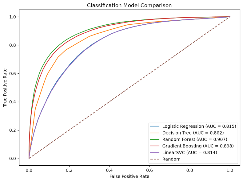
Other metrics such as accuracy, precision, recall, and F1 score were also measured for each model. At the standard classification threshold, the Random Forest model correctly classified about 84% of events, while its precision and recall were approximately 80% and 72%, respectively. These metrics describe a particular operating point, whereas the ROC AUC captures the model's overall ability to rank signal events above background across thresholds.

Looking Inside the Model

A strong classification score tells us that the model can distinguish signal from background, but it does not tell us how it is making those decisions. Since the model was trained on physical measurements, I wanted to look inside it and see which of those measurements were most important to its predictions.

I began by examining the model's feature importance. This provides a first look at which physical observables the Random Forest relied on most heavily when separating signal from background.

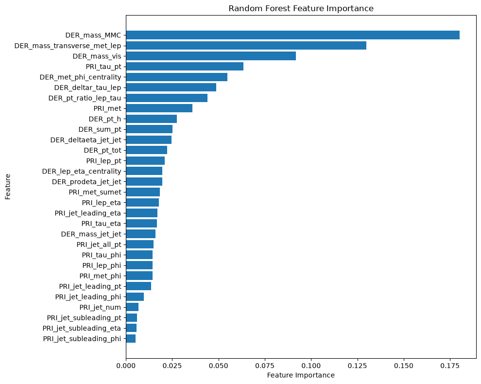
The resulting ranking showed that the model did not treat all of the measurements equally. A relatively small group of observables contributed much more strongly to its predictions than others. This provided a useful connection between the machine learning model and the underlying physics: the classifier was finding structure in specific properties of the collision rather than simply treating every input as equally informative.

Feature importance tells us which variables the model uses, but it does not tell us how those variables influence its predictions. To investigate this, I used partial dependence plots (PDPs).

A PDP shows how the model's prediction changes as one feature is varied while averaging over the other features in the dataset. This provides a way to visualize the relationship the model has learned between a physical observable and its prediction.

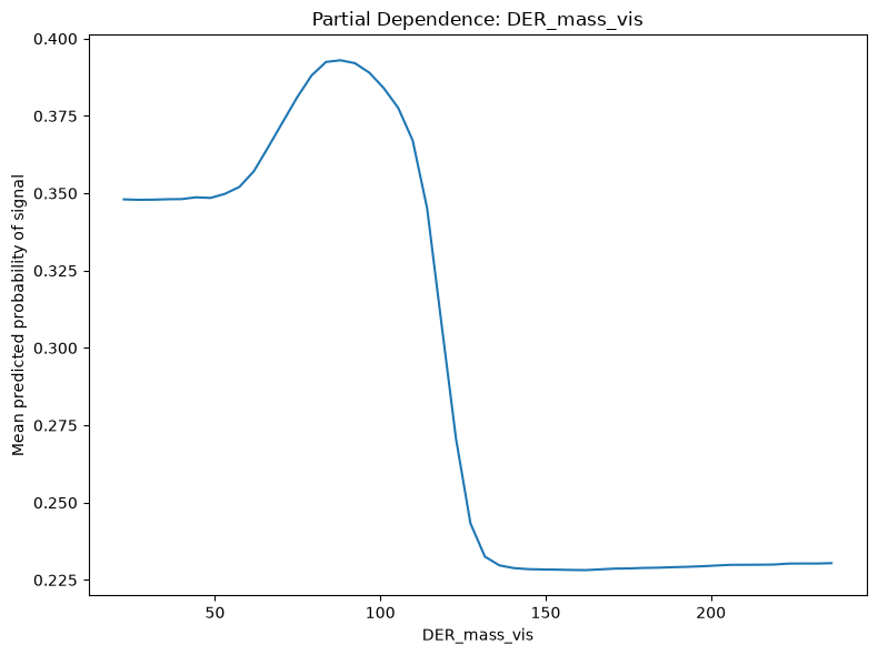
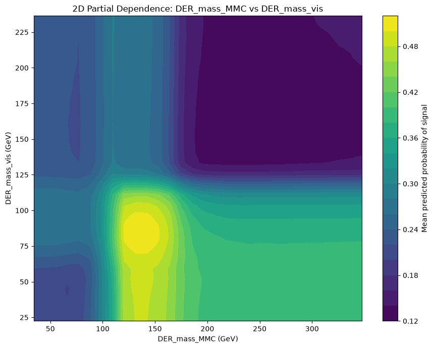
Together, these analyses gave me a way to move beyond simply asking whether the model worked. The Random Forest was not just producing a classification score; its predictions could be investigated in terms of the physical measurements it was given.

What I Learned

This project taught me that building a machine learning model is only one part of a much larger process. Much of the work was in understanding the data, deciding which tests were useful, interpreting the results, and learning when a result was actually telling me something meaningful.

I learned how important it is to properly split data into training and testing sets before evaluating a model, and how different choices in preprocessing can affect the results. Working through several classification methods also showed me that there is no single model that is automatically best for every problem. Comparing Logistic Regression, Decision Trees, Random Forests, Gradient Boosting, and Linear SVMs gave me a much better understanding of what metrics such as accuracy, precision, recall, F1 score, and ROC AUC actually measure and when each one is useful.

I also learned that improving a model can take considerably more time than simply training it once. Testing different Random Forest parameters, evaluating their effects, and balancing computational cost against potential improvements gave me a much better appreciation for the practical side of machine learning. Some experiments produced meaningful improvements, while others changed the result very little. Learning to recognize that difference was just as valuable as finding the final model.

Another major part of the project was learning how to interpret a model rather than treating it as a black box. Feature importance and permutation importance provided different ways of assessing which physical variables were most influential. Correlation analysis and histograms helped me explore relationships within the original data, while partial dependence plots (PDPs) allowed me to visualize how changing individual features affected the model's predictions. I also explored two-dimensional PDPs to investigate how combinations of features influenced the model, and examined different probability thresholds to understand the tradeoff between identifying more signal events and reducing false positives.

What I found most valuable was seeing how these different techniques complemented one another. A histogram could reveal a difference between signal and background that motivated further investigation; feature importance could show that a variable mattered to the model; and a PDP could then provide a visual picture of how the model responded to that variable. Rather than relying on a single number, I learned to use visualizations, statistical measures, model metrics, and physical intuition together to understand what was happening.

Finally, the project gave me experience with something that is difficult to learn from individual examples: working through an open-ended computational problem from beginning to end. Experiments took time, some approaches were less useful than expected, and interpreting a result often required going back and asking a different question. The process taught me not only how to use machine learning techniques, but how to investigate a problem systematically and communicate what I found.

Explore the Technical Work

This page provides an overview of the project and the ideas behind it. The complete technical analysis is available in the project's Jupyter notebooks, including the data exploration, model development, optimization, and model interpretation.